I presented this project as a poster at the CMU Sports Analytics Conference. The full research and associated code and conference poster are available online.
Overview
Since the advent of basketball analytics, a metric that can accurately determine the relative value of a player’s defense has been widely sought after. It is widely regarded that features like shot defense are key to a player’s defensive identity, but regularized on-off metrics like RAPM are unable to take this into account. Using player-tracking data, we are able to extract information about shot defense.
We determine the relative importance of a set of offensive and defensive factors on individual shots near the three-point line. Using 2015-16 SportVU data, where player and ball positional coordinates are captured 25 times a second, and the accompanying play-by-play data, we extract the following features: ‘Distance Between Shooter And Defender’, ‘Shot Distance’, ‘Difference Between Shooter And Defender Height’, and ‘3PT%’. 3PT% is calculated for the entirety of the 2015-16 season.
We then train a gradient boosting model to predict the shot success probability of a given shot. Although this can be useful on its own, it does not directly provide the relative importance of each of the input features.
To this end, we use interpretable machine learning techniques, specifically Shapley values. Using TreeSHAP, we determine the importance scores for each input feature, per shot. Aggregating these values over all games in our dataset, we estimate the relative importance of each feature.
Model
Our preliminary goal is to devise a method to statistically determine the probability of a shot being made. We use XGBoost to model shot probability. Based on a hyperparameter search, we use the following hyperparameters: learning rate=0.05, max depth=3, n estimators=100, basescore=0.45, colsample bytree=1, subsample=0.8, gamma=0. Our chosen booster is ‘gbtree’.
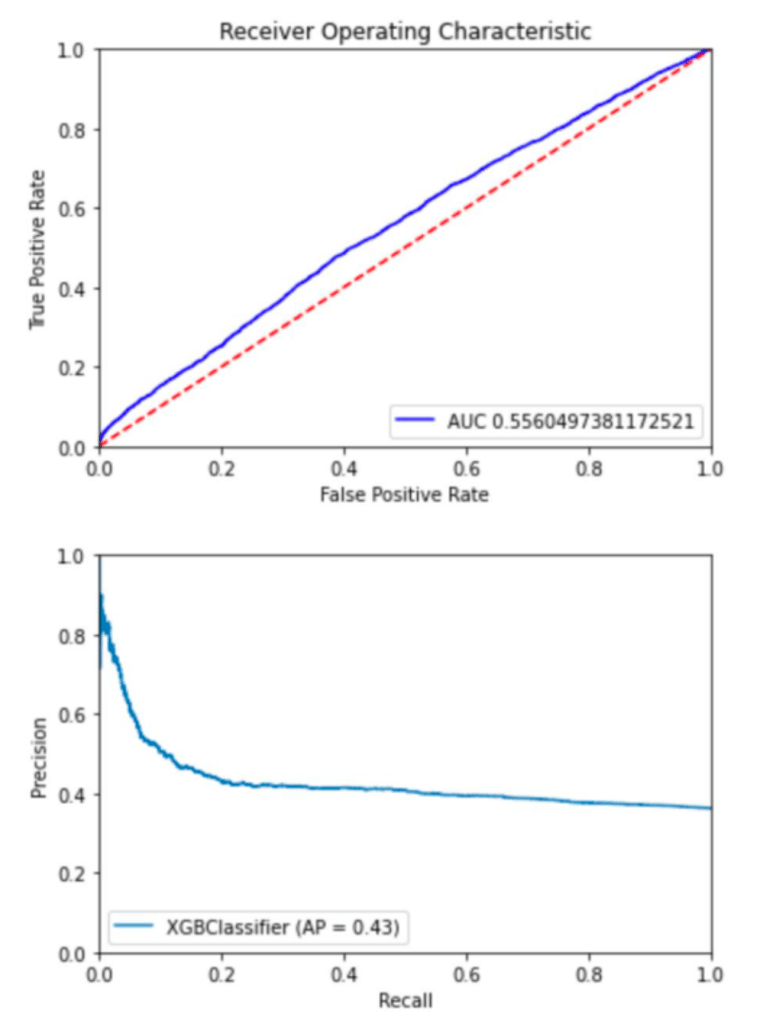
Model Metrics
Although our model’s predictive power isn’t extremely strong (AU-ROC=0.56, AU-PRC=0.43), we still perform better than if we only used 3PT% to make predictions. The league average 3PT% was 0.35, so a random estimator would have an AU-PRC of 0.35. We specifically want to deduce what the model is learning within this improvement above 0.35.
Interpretation
We are then able to interpret the model’s predictions. Specifically, we wish to concretely determine which features the model finds to be the most useful to predict the shot probability.
To this end, we use Shapley values (an idea from cooperative game theory): a concrete way of “splitting up” contributions among features. Shapley values assign specific negative and positive values, which signify whether a trait positively or negatively affects the model’s predictions. The higher the Shapley value for a given feature, the more the model’s prediction was affected by that feature.
In order to solve for our Shapley values, we use TreeSHAP. For each data point (a single shot), we are able to extract the Shapley values for the aforementioned features fed into the model ‘Distance Between Shooter And Defender’, ‘Shot Distance’, ‘Difference Between Shooter And Defender Height’, and ‘3PT%’.
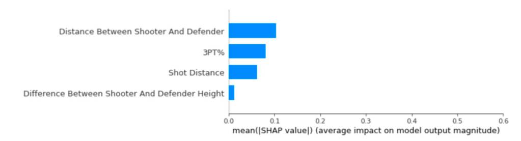
Shapley values summary
In the above plot, we see the average Shapley value for all of the data points. Within this model, the distance between a shooter and their defender is more important than 3PT%, Shot Distance, and the Difference Between Shooter and Defender Height. The difference between a shooter’s height and a defender’s height has little influence on this model’s predictions. Finally, Shot Distance on a 3PT shot appears to be less important to the model than Distance Between Shooter and Defender and the shooter’s 3PT%.
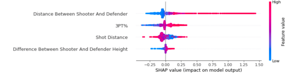
In the more detailed version of our Shapley value plot, we are able to pinpoint the trends for each of the features. For instance, in the 3PT% plot, we notice that the higher the 3PT%, the higher the Shapley value. Although this specific information is fairly intuitive, it serves as a sanity check for what our model learned. Similarly, we can determine the distribution of Shapley values. For instance, there is not much variance in the Shapley values for ‘Difference Between Shooter and Defender Height’, while there is significant variance in ‘Distance Between Shooter and Defender’.
Discussion/Conclusion
This project shows how Shapley values can help us understand which features drive a shot-probability model’s predictions. The results describe this model rather than the causal effect of each feature or the defensive value of individual players. Our approach is similar to Matt Ploenzke’s submission to the Big Data Bowl and demonstrates the potential of interpretable machine learning in sports. Future improvements include strengthening model performance and comparing our shot-probability model with existing models.